Verification studies

Seven studies that measure the machinery rather than any application. Six of them write an artifact that experiments/collect_results.py reads into results, so no number is retyped by hand; the seventh, study_design_table.py, writes design_table.json for the four-row design table below.

Solver and gradient

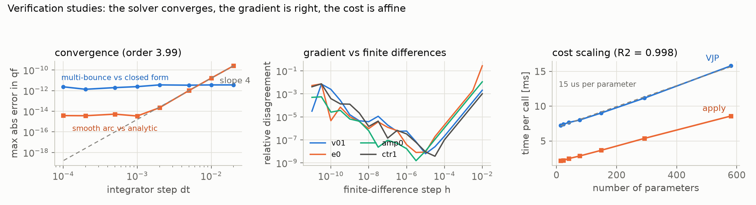
Plotted from convergence_result.npz, gradient_accuracy_result.npz and scaling_result.npz by make_study_figures.py.

Convergence. Order 3.99 on a smooth arc measured against the analytic drag solution. The multi-bounce flat case sits at 10⁻¹² against the symbolic closed form, where the floor is event localization rather than the integrator.

Gradient accuracy. Agreement with central differences traces the expected V in the step size on all four probes, bottoming below 10⁻⁸. This is a falsification test rather than a spot check: a wrong analytic gradient produces a flat floor instead of a V, because the disagreement would be dominated by the gradient error rather than by the step.

Cost scaling. Affine in parameter count out to 581 parameters, 15 microseconds per parameter, R² = 0.998. The slope is wall-clock on one shared laptop and moves between runs: a repeat measured 14.4 microseconds per parameter at R² = 0.9976, a 3.9% spread. The affine shape is what holds.

This slope used to be 93 microseconds, and the difference is not a faster machine. The flow is affine in the state, so the RK4 variational update collapses exactly to a fixed tangent map; propagating that instead of running RK4 on the sensitivity matrix takes the parameter dimension out of the inner loop. What is left is the per-event work.

Optimizer benchmark

A single run from one start point cannot support a claim about methods, so this repeats the 24-dimensional design from five random starts with both methods tuned over a grid per seed, learning rate for Adam and sigma0 for CMA-ES.

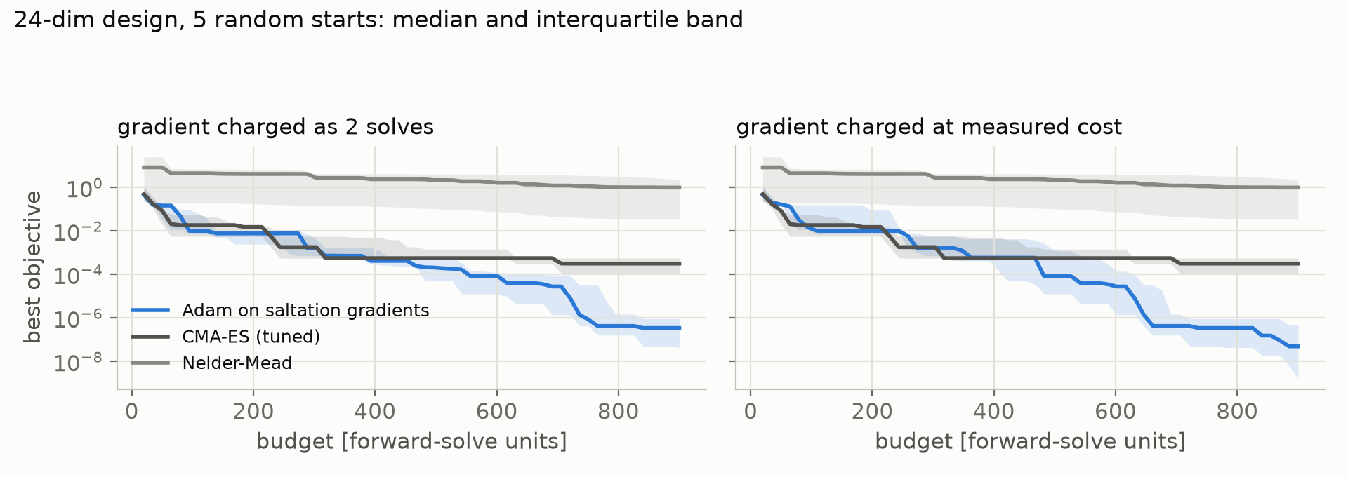
Plotted from optimizer_benchmark.npz by make_study_figures.py.

Per evaluation, gradients win decisively: median final objective 3.4×10⁻⁷ for Adam against 3.2×10⁻⁴ for tuned CMA-ES. The seeds are paired, so the honest statistic is the median of the per-seed ratios, 347x, rather than the ratio of the medians; and the per-seed ratios span 12x to 139843x, so the direction is unanimous across five seeds but the magnitude is not resolvable at this sample size. Nelder-Mead sits a further 3.5 orders behind CMA-ES.

Charged by measured wall-clock the picture used to be worse for Adam, and this is the honest history. When a gradient call cost a measured 6.8 forward solves, CMA-ES was ahead on 4 of 5 seeds, a sign test gave p = 0.375, and a bootstrap interval on the median per-seed ratio spanned both sides of parity; we reported that the wall-clock ordering was unresolved rather than reversed. That 6.8 was an artifact of how the solver propagated sensitivities, not a property of saltation gradients. The flow is affine in the state, so the RK4 variational update collapses to a fixed tangent map that can be composed across a smooth segment; with that factoring a gradient costs 1.612 solves and Adam is ahead on all five seeds.

Read that carefully: we made our own gradient cheaper and the accounting followed. It is evidence about this implementation, not about gradient methods against gradient-free ones, and the E5b control below is where that second question actually gets answered.

Important

The wall-clock accounting is reported rather than hidden. What it exposed was an implementation property, not a fact about gradients, and we then fixed the implementation. The VJP is still forward-variational and still carries one column per parameter, but the per-step work no longer touches the parameter dimension; what is left is the per-event work, at 15 microseconds per parameter. A reverse-mode saltation adjoint remains the right extension for large state dimension rather than for large parameter count.

What does not change under either accounting is the objective value: at 24 dimensions the gradient-free methods plateau 1.1 to 8.0 orders above what Adam attains per evaluation.

Important

That gap does not survive translation into engineering units, and we checked rather than assumed. The loss is squared landing error summed over two particles, so Adam’s 2.25e-07 is a 0.34 mm miss, while the CMA-ES design that E5b actually scores sits at 1.98e-03, about 31 mm per particle. The bins are 1600 mm apart. Scoring all four designs on the held-out scatter ensemble that E5b uses:

design	purity (95% Wilson)	5th-percentile margin, m (95% bootstrap)
Adam	199/200 (97–100%)	+0.07 (+0.06 to +0.32)
CMA-ES	196/200 (95–99%)	+0.18 (+0.11 to +0.25)
Nelder-Mead	199/200 (97–100%)	+0.41 (+0.33 to +0.52)
ensemble-refined	200/200 (98–100%)	+0.43 (+0.40 to +0.52)

All four are scored on the same 200 particles, so the columns are paired. The intervals come from experiments/study_design_table.py into design_table.json: Wilson on the purities, and 10,000 bootstrap resamples at a pinned seed on the fifth percentile. The purity intervals overlap for every pair, so purity does not separate these designs at this sample size; the margin intervals separate Adam from both Nelder-Mead and the ensemble design, and do not separate those two from each other.

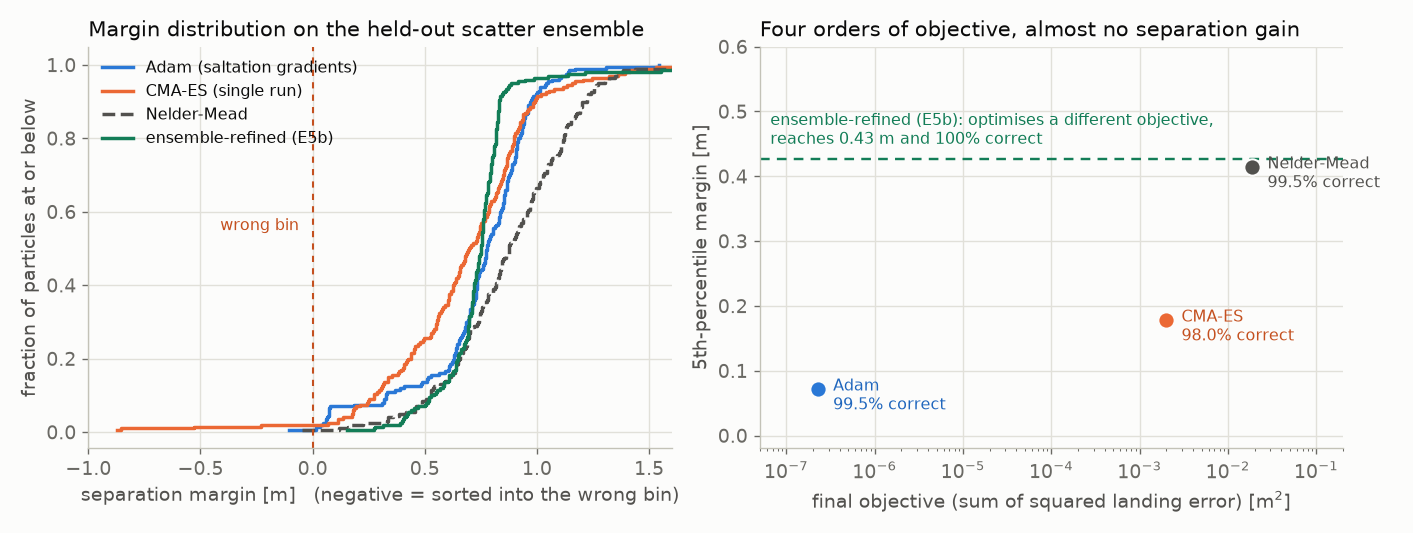
Plotted from e5b_result.npz and e5_result.npz by make_design_comparison_figure.py.

Nelder-Mead is five orders behind on the objective and sorts exactly as well as Adam, with a wider margin. Minimising the point objective further does not buy a better separator at this scale. Optimising the ensemble objective does separate from Adam, whose margin interval it clears. It does not separate from Nelder-Mead on the margin: those two intervals overlap, and on this ensemble the honest claim stops there.

We used to say the ensemble objective was where the gradient pays, because it needs a gradient through many trajectories at once. That was asserted, and when we finally measured it the claim did not survive. See the control below: what buys the robustness is optimising the ensemble objective at all, not the gradient that does it.

The control: gradient-free on the ensemble objective

For most of this project the answer to “Nelder-Mead matches Adam on held-out purity” was that the ensemble objective is different, and that it needs a gradient through many trajectories at once. Nobody had run a gradient-free method on the ensemble objective, so the sentence was an assertion. We ran it.

Same warm start as E5b, same training draw, same held-out ensemble, same objective. The budget is matched in particle solves: an Adam step issues an apply and a vector_jacobian_product per particle, and the measured gradient charge is the reverse pass alone, so a step costs (1 + charge) per particle. That is 5040 solves, or 210 gradient-free ensemble evaluations. CMA-ES was swept over three initial step sizes and three seeds, because e5_cma_grid.py had already measured a 24x spread across that grid and one hardcoded configuration would have decided the result by the protocol. Nelder-Mead got an explicit initial simplex at two scales, because scipy’s default builds it as x_i * 1.05, which from this warm start spans four orders of magnitude and freezes the small amplitudes.

method	ensemble objective	held-out	5th-percentile margin
warm start (E5 point design)	7.3e-2	199/200	+0.07 m
Adam, published lr = 0.004	0.01831281	200/200	+0.426 m
Adam, best of 5 learning rates	0.01210364	200/200	+0.6004 m
CMA-ES, best of 9	0.00735504	200/200	+0.5584 m
Nelder-Mead, best of 2	0.0266707	188/200	-0.005 m

Important

The claim did not survive. CMA-ES reaches a better ensemble design than the published Adam run at a matched budget, on the objective and on the tail, and it beats that run’s objective on every one of its 9 grid runs; its median, 0.01187285, still beats Adam’s best. Because the first comparison gave CMA-ES nine configurations and Adam one, we then swept Adam’s learning rate over 5 values fixed before the run. The objective ordering is unchanged, and the sweep turns up two things: the published lr = 0.004 is not Adam’s best here, lr = 0.001 reaches 0.01210364; and the tail ordering does not hold up, since that run’s fifth-percentile margin is +0.6004 m against CMA-ES’s +0.5584 m. CMA-ES wins the objective; on the tail the two do not separate.

Does the concession hold at more design variables?

Twenty-four parameters is where CMA-ES is comfortable, and the cost scaling above says the gradient’s per-step work does not grow with the parameter count. So we re-ran the same comparison at 93.

The experiment only means anything if raising the count raises the dimension and not the difficulty, so the design space is nested by construction. A wide Gaussian is a positive convolution of narrow ones, so with bump width scaled to spacing the published 24-parameter design is an exact interior point of the 93-parameter box: it reproduces the same trajectory impact for impact, with identical status and event counts on all 24 training particles, and the warm start moves the objective by 0.4%. Therefore the best achievable loss at 93 is no worse than at 24 by construction, and any degradation measured is the optimiser failing rather than the problem hardening. The evaluation budget is frozen at 315 ensemble evaluations at both dimensions, and both arms’ step-size grids are recalibrated by the same measured rule, because a step in absolute amplitude units means something different when bumps are four times narrower.

design variables	Adam best	CMA-ES best	CMA / Adam, best	CMA / Adam, median
24	0.01026725	0.00647431	0.631	0.577
93	0.00399458	0.01507056	3.773	1.462

At 93 parameters CMA-ES given 3 times the budget reaches 0.01083864, still 2.71 times Adam’s matched-budget result, so this is not starvation.

Important

The concession we published stands at 24 design variables and does not extend to 93 on this problem. That is the honest shape of it: gradient-free search wins where the design space is small, and stops winning as it grows, which is what the cost scaling predicts and is why the gradient is worth having.

The limits matter as much as the result. This is two dimension points on one problem instance with one training draw, so it does not estimate a crossover dimension and says nothing about other objectives or budget levels. The objective has 48 residuals, which caps its local rank whatever the parameter count is, so 93 parameters is an over-parameterised design vector rather than 93 independent degrees of freedom. A pre-registered middle point at 47 was dropped on its own gate, not accommodated: the embedded warm start moved the objective 10.1% there against a 5% threshold, because 47 bumps do not yet represent the 24-bump terrain faithfully.

CMA-ES’s best configuration at 24 sat on the edge of its step-size grid, so the grid was extended one step, which could only have strengthened the concession against us. It did not improve: 1.45e-2 against 6.47e-3.

None of this touches E2b, where the gradient is not a faster route to the same answer but the only route to any: NUTS calls for a gradient at every one of its 23,440 leapfrog steps, and no gradient-free method samples that posterior at all. The comparisons above are about search on a 24-dimensional design; that one is about whether the problem is reachable.

So the honest statement is that optimising the ensemble objective is what buys the robustness, and the gradient is not what makes that possible. Nelder-Mead is genuinely worse, so this is not “gradient-free wins”; it is CMA-ES being well suited to a 24-dimensional box with a good warm start.

What remains true of the gradient is cost per step, not reachability, and this project has not measured that cleanly enough to lead with it.

Robustness and generalization

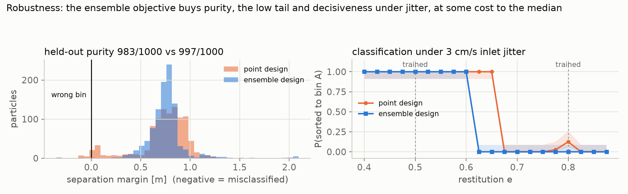
Plotted from robustness_stats.npz and generalization_stats.npz by make_study_figures.py.

Purity with intervals. Over five independent 200-particle ensembles the point design classifies 983 of 1000 and the ensemble design 997 of 1000, with non-overlapping Wilson intervals. More useful than the headline percentage is the separation margin: its fifth percentile improves from 0.05 m to 0.49 m (paired bootstrap 95% interval [+0.39, +0.47] m). The worst case does not improve: it goes from -0.12 m to -0.35 m, both inside the wrong bin. The ensemble objective buys the low tail, not the extreme, and it pays in the centre: the median margin drops 2.7 cm, with a paired 95% interval of [-0.040, -0.009] m that excludes zero.

Decisiveness under jitter. Sweeping restitution with inlet jitter shows what the deterministic sweep hid. The point design is indecisive at 2 of 20 restitutions, including its own trained value of 0.8, where 12.5% of jittered draws cross into the wrong bin. The ensemble design is decisive at all 20.

Two honest limits on that. The designs are scored on the same restitutions and the same jitter draws, so the comparison is paired: two discordant restitutions against none, and exact McNemar gives p = 0.50, the smallest value two discordant pairs can produce. The direction is consistent and the failure at the trained value is real, but this comparison has no power to establish it. And decisiveness means 0 failures in 40 draws per restitution, which bounds the per-restitution failure rate at about 7.5%, not at zero.